Regional Amplification of Global Warming: Do the Models Get It Right?
Warming at the Poles Since 1950
Figure 52. The above figure shows the polar amplification for both Antarctica and the Arctic. The ratio is computed by comparing the warming trends seen at each pole compared to the average global trend. The points are the observed Berkeley Earth data shown in red, and the GCMs (Global Climate Models) shown in blue. The models tend to overestimate the warming in the Arctic and in Antarctica. The period 1950-to-present is shown because Antarctica has no data prior to this period. Polar amplification results in part because of feedbacks from melting ice and reduced snow cover in a warming world, causing the region to absorb more of the sun’s energy rather than reflect it back to outer space.
Figure 53. This figure shows the amplification ratio between 30N and 60N (roughly from the middle of Texas to the bottom tip of Greenland) compared to the amplification ratio in the Arctic. The observed value from Berkeley Earth is shown in red and the GCMs are in blue. The GCMs tend to overestimate the amplification at the pole and underestimate the amplification in the mid-latitudes.
Figure 54. This plot gives an idea of the degree to which GCM radiative forcing behavior in the 21st century is predicted to be the same as that during the 20th century. Each dot represents a GCM model. Models that plot near the x = y line are ones where the 21st century and the past have similar responses to forcing. Those that plot above the line are predicting that the future warming will be larger than one might predict based in the 20th century response characteristics. As can be seen, about 60% of the GCMs show some degree of acceleration in their response. In a few cases, the predicted future response is 2 or 3 times that demonstrated during the recent past. The phrase “response to radiative forcing” refers to the planet’s temperature change for a given increase in greenhouse gases.
How Good Are The Models? Berkeley Earth Check on 20th Century Model Performance
AR4 GCMs versus BE Dataset
Figure 9. The above figure shows a comparison between the Berkeley Earth Surface Air Temperature record and a collection of GCM results from the IPCC’s AR4 report. The GCM results were created by sampling the entire GCM field at the same locations and times as the Berkeley Earth average. The GCM average is shown in red and the Berkeley average is shown in black.
Many Models Still Struggle With Overall Warming; None Replicate Regional Warming Well
The following graphics show the land surface temperature results derived from Berkeley Earth’s computations versus the output of a series climate models. In the literature these models are referred to as Global Climate Models or “GCMs.” Climate models are computer simulations which attempt to mathematically reproduce the Earth’s climate, and are used by some scientists studying climate change to attempt to understand the future timing, magnitude, and effects of global warming.
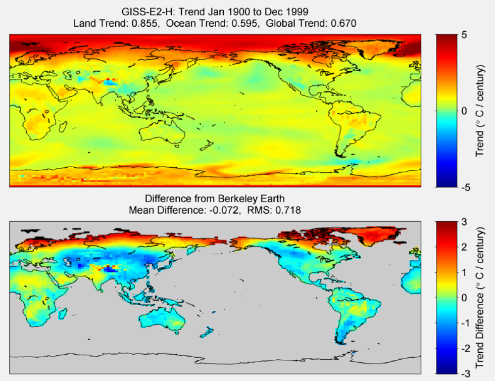
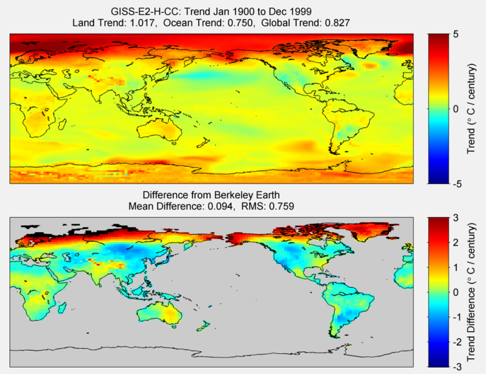
The top portion of each graphic shows the warming trends (degrees C per century) over land, ocean, and global areas for the referenced model. The bottom portion of each graphic shows the difference between the model results and the actual historical temperature map derived from the Berkeley Earth land-based dataset. A model which perfectly replicates the historical temperature trend for all regions of the globe would show a uniform green color (the color for zero difference in temperature trend between the model and the historical record) for all land areas. The yellow/red range of the color scale indicates model temperature trends which overstate (are higher than) the actual historical trend for a region. The blue range of the color scale indicates model temperature trends which understate (are lower than) the actual historical trend for a region. NASA’s “GISS-E2-H” model appears to replicate overall warming best, but is among the worst models at replicating regional trends. China’s “FGOALS-g2” appears to be the best performer at replicating regional trends, but still over/under-predicts the warming trend by about 0.5C per century almost everywhere.
Figure 46. The above graphic illustrates the 100-year trend from 1900 to 1999 for the historical reconstruction produced as part of the Coupled Model Intercomparson project –Phase 5 or CMIP 5. Results for the MPI-ESM-MR model are shown in the upper panel, and the difference with Berkeley Earth land temperatures is shown in the lower panel. MPI-ESM-MR is a product of the Max-Planck-Institut für Meteorologie (Max Planck Institute for Meteorology). The lower panel depicts the difference in trends between MPI-ESM-MR and Berkeley Earth land temperatures. The Root Mean Square (RSM) is calculated at the grid level.
Figure 12. The above graphic illustrates the 100 year trend from 1900 to 1999 for the historical reconstruction produced as part of the Coupled Model Intercomparson project –Phase 5 or CMIP 5. Results for the ACCESS1-0 model is shown in the upper panel and the difference with Berkeley Earth Land Temperature is shown in the lower panel. ACCESS1-0 is a product of Commonwealth Scientific and Industrial Research Organization (CSIRO) and Bureau of Meteorology (BOM), Australia. The lower panel depicts the difference in trends between ACCESS1-0 and Berkeley Earth Surface Temperatures. The Root Mean Square is calculated at the grid level.
Figure 13. The above graphic illustrates the 100 year trend from 1900 to 1999 for the historical reconstruction produced as part of the Coupled Model Intercomparson project –Phase 5 or CMIP 5. Results for the ACCESS1-3 model is shown in the upper panel and the difference with Berkeley Earth Land Temperature is shown in the lower panel. ACCESS1-3 is a product of Commonwealth Scientific and Industrial Research Organization (CSIRO) and Bureau of Meteorology (BOM), Australia. The lower panel depicts the difference in trends between ACCESS1-3 and Berkeley Earth Surface Temperatures. The Root Mean Square is calculated at the grid level.
Figure 14. The above graphic illustrates the 100 year trend from 1900 to 1999 for the historical reconstruction produced as part of the Coupled Model Intercomparson project –Phase 5 or CMIP 5. Results for bcc-csm1-1 model is shown in the upper panel and the difference with Berkeley Earth Land Temperature is shown in the lower panel. Bcc-csm1-1 is a product of a product of Beijing Climate Center, China Meteorological Administration. The lower panel depicts the difference in trends between Bcc-csm1-1 and Berkeley Earth Land Temperatures. The Root Mean Square is calculated at the grid level.
Figure 15. The above graphic illustrates the 100 year trend from 1900 to 1999 for the historical reconstruction produced as part of the Coupled Model Intercomparson project –Phase 5 or CMIP 5. Results for bcc-csm1-1m model is shown in the upper panel and the difference with Berkeley Earth Land Temperature is shown in the lower panel. Bcc-csm1-1 is a product of a product of Beijing Climate Center, China Meteorological Administration. The lower panel depicts the difference in trends between Bcc-csm1-1m and Berkeley Earth Land Temperatures. The Root Mean Square is calculated at the grid level.
Figure 16. The above graphic illustrates the 100 year trend from 1900 to 1999 for the historical reconstruction produced as part of the Coupled Model Intercomparson project –Phase 5 or CMIP 5. Results for CanESM2 model is shown in the upper panel and the difference with Berkeley Earth Land Temperature is shown in the lower panel. CanESM2 is a product of the Canadian Centre for Climate Modelling and Analysis. The lower panel depicts the difference in trends between CanESM2 and Berkeley Earth Land Temperatures. The Root Mean Square is calculated at the grid level.
Figure 17. The above graphic illustrates the 100 year trend from 1900 to 1999 for the historical reconstruction produced as part of the Coupled Model Intercomparson project –Phase 5 or CMIP 5. Results for CCSM4 model is shown in the upper panel and the difference with Berkeley Earth Land Temperature is shown in the lower panel. CCSM4 is a product of the National Center for Atmospheric Research (NCAR) . The lower panel depicts the difference in trends between CCSM4 and Berkeley Earth Land Temperatures. The Root Mean Square is calculated at the grid level.
Figure 18. The above graphic illustrates the 100 year trend from 1900 to 1999 for the historical reconstruction produced as part of the Coupled Model Intercomparson project –Phase 5 or CMIP 5. Results for CESM1-BGC model is shown in the upper panel and the difference with Berkeley Earth Land Temperature is shown in the lower panel. CESM1-BGC is a product of the Community Earth System Model Contributors (NSF,DEO & NCAR) . The lower panel depicts the difference in trends between CESM1-BGC and Berkeley Earth Land Temperatures. The Root Mean Square is calculated at the grid level.
Figure 19. The above graphic illustrates the 100 year trend from 1900 to 1999 for the historical reconstruction produced as part of the Coupled Model Intercomparson project –Phase 5 or CMIP 5. Results for CESM1-CAM5 model is shown in the upper panel and the difference with Berkeley Earth Land Temperature is shown in the lower panel. CESM1-CAM5 is a product of the Community Earth System Model Contributors (NSF,DEO & NCAR) . The lower panel depicts the difference in trends between CESM1-CAM5 and Berkeley Earth Land Temperatures. The Root Mean Square is calculated at the grid level.
Figure 20. The above graphic illustrates the 100 year trend from 1900 to 1999 for the historical reconstruction produced as part of the Coupled Model Intercomparson project –Phase 5 or CMIP 5. Results for CESM1-FASTCHEM model is shown in the upper panel and the difference with Berkeley Earth Land Temperature is shown in the lower panel. CESM1-FASTCHEM is a product of the Community Earth System Model Contributors (NSF,DEO & NCAR) . The lower panel depicts the difference in trends between CESM1-FASTCHEM and Berkeley Earth Land Temperatures. The Root Mean Square is calculated at the grid level.
Figure 21. The above graphic illustrates the 100 year trend from 1900 to 1999 for the historical reconstruction produced as part of the Coupled Model Intercomparson project –Phase 5 or CMIP 5. Results for CESM1-WACCM model is shown in the upper panel and the difference with Berkeley Earth Land Temperature is shown in the lower panel. CESM1-WACCM is a product of the Community Earth System Model Contributors (NSF,DEO & NCAR) . The lower panel depicts the difference in trends between CESM1-WACCM and Berkeley Earth Land Temperatures. The Root Mean Square is calculated at the grid level.
Figure 22. The above graphic illustrates the 100 year trend from 1900 to 1999 for the historical reconstruction produced as part of the Coupled Model Intercomparson project –Phase 5 or CMIP 5. Results for CMCC-CESM model is shown in the upper panel and the difference with Berkeley Earth Land Temperature is shown in the lower panel. CMCC-CESM is a product of Centro Euro-Mediterraneo per I Cambiamenti Climatici. The lower panel depicts the difference in trends between CMCC-CESM and Berkeley Earth Land Temperatures. The Root Mean Square is calculated at the grid level.
Figure 23. The above graphic illustrates the 100 year trend from 1900 to 1999 for the historical reconstruction produced as part of the Coupled Model Intercomparson project –Phase 5 or CMIP 5. Results for CMCC-CM model is shown in the upper panel and the difference with Berkeley Earth Land Temperature is shown in the lower panel. CMCC-CM is a product of Centro Euro-Mediterraneo per I Cambiamenti Climatici. The lower panel depicts the difference in trends between CMCC-CM and Berkeley Earth Land Temperatures. The Root Mean Square is calculated at the grid level.
Figure 24. The above graphic illustrates the 100 year trend from 1900 to 1999 for the historical reconstruction produced as part of the Coupled Model Intercomparson project –Phase 5 or CMIP 5. Results for CMCC-CMS model is shown in the upper panel and the difference with Berkeley Earth Land Temperature is shown in the lower panel. CMCC-CMS is a product of Centro Euro-Mediterraneo per I Cambiamenti Climatici. The lower panel depicts the difference in trends between CMCC-CMS and Berkeley Earth Land Temperatures. The Root Mean Square is calculated at the grid level.
Figure 25. The above graphic illustrates the 100 year trend from 1900 to 1999 for the historical reconstruction produced as part of the Coupled Model Intercomparson project –Phase 5 or CMIP 5. Results for CNRM-CM5-2 model is shown in the upper panel and the difference with Berkeley Earth Land Temperature is shown in the lower panel. CNRM-CM5-2 is a product of CCentre National de Recherches Météorologiques / Centre Européen de Recherche et Formation Avancée en Calcul Scientifique. The lower panel depicts the difference in trends between CNRM-CM5-2 and Berkeley Earth Land Temperatures. The Root Mean Square is calculated at the grid level.
Figure 26. The above graphic illustrates the 100 year trend from 1900 to 1999 for the historical reconstruction produced as part of the Coupled Model Intercomparson project –Phase 5 or CMIP 5. Results for CNRM-CM5 model is shown in the upper panel and the difference with Berkeley Earth Land Temperature is shown in the lower panel. CNRM-CM5 is a product of CCentre National de Recherches Météorologiques / Centre Européen de Recherche et Formation Avancée en Calcul Scientifique. The lower panel depicts the difference in trends between CNRM-CM5 and Berkeley Earth Land Temperatures. The Root Mean Square is calculated at the grid level.
Figure 27. The above graphic illustrates the 100 year trend from 1900 to 1999 for the historical reconstruction produced as part of the Coupled Model Intercomparson project –Phase 5 or CMIP 5. Results for CSIRO-Mk3-6-0 model is shown in the upper panel and the difference with Berkeley Earth Land Temperature is shown in the lower panel. CSIRO-Mk3-6-0 is a product of Commonwealth Scientific and Industrial Research Organization in collaboration with Queensland Climate Change Centre of Excellence. The lower panel depicts the difference in trends between CSIRO-Mk3-6-0 and Berkeley Earth Land Temperatures. The Root Mean Square is calculated at the grid level.
Figure 28. The above graphic illustrates the 100 year trend from 1900 to 1999 for the historical reconstruction produced as part of the Coupled Model Intercomparson project –Phase 5 or CMIP 5. Results for FGOALS-g2 model is shown in the upper panel and the difference with Berkeley Earth Land Temperature is shown in the lower panel. FGOALS-g2 is a product of LASG, Institute of Atmospheric Physics, Chinese Academy of Sciences and CESS,Tsinghua University. The lower panel depicts the difference in trends between FGOALS-g2 and Berkeley Earth Land Temperatures. The Root Mean Square is calculated at the grid level.
Figure 29. The above graphic illustrates the 100 year trend from 1900 to 1999 for the historical reconstruction produced as part of the Coupled Model Intercomparson project –Phase 5 or CMIP 5. Results for FIO-ESM model is shown in the upper panel and the difference with Berkeley Earth Land Temperature is shown in the lower panel. FIO-ESM is a product of The First Institute of Oceanography, SOA, China. The lower panel depicts the difference in trends between FIO-ESM and Berkeley Earth Land Temperatures. The Root Mean Square is calculated at the grid level.
Figure 30. The above graphic illustrates the 100 year trend from 1900 to 1999 for the historical reconstruction produced as part of the Coupled Model Intercomparson project –Phase 5 or CMIP 5. Results for GFDL-CMP2.1 model is shown in the upper panel and the difference with Berkeley Earth Land Temperature is shown in the lower panel. GFDL-CMP2.1 is a product of NOAA Geophysical Fluid Dynamics Laboratory. The lower panel depicts the difference in trends between GFDL-CMP2.1 and Berkeley Earth Land Temperatures. The Root Mean Square is calculated at the grid level.
Figure 31. The above graphic illustrates the 100 year trend from 1900 to 1999 for the historical reconstruction produced as part of the Coupled Model Intercomparson project –Phase 5 or CMIP 5. Results for GFDL-CM3 model is shown in the upper panel and the difference with Berkeley Earth Land Temperature is shown in the lower panel. GFDL-CM3 is a product of NOAA Geophysical Fluid Dynamics Laboratory. The lower panel depicts the difference in trends between GFDL-CMP3 and Berkeley Earth Land Temperatures. The Root Mean Square is calculated at the grid level.
Figure 32. The above graphic illustrates the 100 year trend from 1900 to 1999 for the historical reconstruction produced as part of the Coupled Model Intercomparson project –Phase 5 or CMIP 5. Results for GFDL-ESM2M model is shown in the upper panel and the difference with Berkeley Earth Land Temperature is shown in the lower panel. GFDL-ESM2M is a product of NOAA Geophysical Fluid Dynamics Laboratory. The lower panel depicts the difference in trends between GFDL-ESM2M and Berkeley Earth Land Temperatures. The Root Mean Square is calculated at the grid level.
Figure 33. The above graphic illustrates the 100 year trend from 1900 to 1999 for the historical reconstruction produced as part of the Coupled Model Intercomparson project –Phase 5 or CMIP 5. Results for GISS-E2-H model is shown in the upper panel and the difference with Berkeley Earth Land Temperature is shown in the lower panel. GISS-E2-H is a product of NASA Goddard Institute for Space Studies. The lower panel depicts the difference in trends between GISS-E2-H and Berkeley Earth Land Temperatures. The Root Mean Square is calculated at the grid level.
Figure 34. The above graphic illustrates the 100 year trend from 1900 to 1999 for the historical reconstruction produced as part of the Coupled Model Intercomparson project –Phase 5 or CMIP 5. Results for GISS-E2-H-CC model is shown in the upper panel and the difference with Berkeley Earth Land Temperature is shown in the lower panel. GISS-E2-H-CC is a product of NASA Goddard Institute for Space Studies. The lower panel depicts the difference in trends between GISS-E2-H-CC and Berkeley Earth Land Temperatures. The Root Mean Square is calculated at the grid level.
Figure 35. The above graphic illustrates the 100 year trend from 1900 to 1999 for the historical reconstruction produced as part of the Coupled Model Intercomparson project –Phase 5 or CMIP 5. Results for GISS-E2-R model is shown in the upper panel and the difference with Berkeley Earth Land Temperature is shown in the lower panel. GISS-E2-R is a product of NASA Goddard Institute for Space Studies. The lower panel depicts the difference in trends between GISS-E2-R and Berkeley Earth Land Temperatures. The Root Mean Square is calculated at the grid level.
Figure 36. The above graphic illustrates the 100 year trend from 1900 to 1999 for the historical reconstruction produced as part of the Coupled Model Intercomparson project –Phase 5 or CMIP 5. Results for GISS-E2-R-CC model is shown in the upper panel and the difference with Berkeley Earth Land Temperature is shown in the lower panel. GISS-E2-R-CC is a product of NASA Goddard Institute for Space Studies. The lower panel depicts the difference in trends between GISS-E2-R-CC and Berkeley Earth Land Temperatures. The Root Mean Square is calculated at the grid level.
Figure 37. The above graphic illustrates the 100 year trend from 1900 to 1999 for the historical reconstruction produced as part of the Coupled Model Intercomparson project –Phase 5 or CMIP 5. Results for HadGEM2-AO model is shown in the upper panel and the difference with Berkeley Earth Land Temperature is shown in the lower panel. HadGEM2-AO is a product of National Institute of Meteorological Research/KoreaMeteorological Administration. The lower panel depicts the difference in trends between HadGEM2-AO and Berkeley Earth Land Temperatures. The Root Mean Square is calculated at the grid level.
Figure 38. The above graphic illustrates the 100 year trend from 1900 to 1999 for the historical reconstruction produced as part of the Coupled Model Intercomparson project –Phase 5 or CMIP 5. Results for INMCM4 model is shown in the upper panel and the difference with Berkeley Earth Land Temperature is shown in the lower panel. INMCM4 is a product of the Institute for Numerical Mathematics. The lower panel depicts the difference in trends between INMCM4 and Berkeley Earth Land Temperatures. The Root Mean Square is calculated at the grid level.
Figure 39. The above graphic illustrates the 100 year trend from 1900 to 1999 for the historical reconstruction produced as part of the Coupled Model Intercomparson project –Phase 5 or CMIP 5. Results for IPSL-CM5A-LR model is shown in the upper panel and the difference with Berkeley Earth Land Temperature is shown in the lower panel. IPSL-CM5A-LR is a product of the Institut Pierre-Simon Laplace. The lower panel depicts the difference in trends between IPSL-CM5A-LR and Berkeley Earth Land Temperatures. The Root Mean Square is calculated at the grid level.
Figure 40. The above graphic illustrates the 100 year trend from 1900 to 1999 for the historical reconstruction produced as part of the Coupled Model Intercomparson project –Phase 5 or CMIP 5. Results for IPSL-CM5A-MR model is shown in the upper panel and the difference with Berkeley Earth Land Temperature is shown in the lower panel. IPSL-CM5A-MR is a product of the Institut Pierre-Simon Laplace. The lower panel depicts the difference in trends between IPSL-CM5A-MR and Berkeley Earth Land Temperatures. The Root Mean Square is calculated at the grid level.
Figure 41. The above graphic illustrates the 100 year trend from 1900 to 1999 for the historical reconstruction produced as part of the Coupled Model Intercomparson project –Phase 5 or CMIP 5. Results for IPSL-CM5B-MR model is shown in the upper panel and the difference with Berkeley Earth Land Temperature is shown in the lower panel. IPSL-CM5B-MR is a product of the Institut Pierre-Simon Laplace. The lower panel depicts the difference in trends between IPSL-CM5B-MR and Berkeley Earth Land Temperatures. The Root Mean Square is calculated at the grid level.
Figure 42. The above graphic illustrates the 100 year trend from 1900 to 1999 for the historical reconstruction produced as part of the Coupled Model Intercomparson project –Phase 5 or CMIP 5. Results for MIROC5 model is shown in the upper panel and the difference with Berkeley Earth Land Temperature is shown in the lower panel. MIROC5 is a product of the Atmosphere and Ocean Research Institute (The University of Tokyo), National Institute for Environmental Studies, and Japan Agency for Marine-Earth Science and Technology. The lower panel depicts the difference in trends between MIROC5 and Berkeley Earth Land Temperatures. The Root Mean Square is calculated at the grid level.
Figure 43. The above graphic illustrates the 100 year trend from 1900 to 1999 for the historical reconstruction produced as part of the Coupled Model Intercomparson project –Phase 5 or CMIP 5. Results for MIROC-ESM model is shown in the upper panel and the difference with Berkeley Earth Land Temperature is shown in the lower panel. MIROC-ESM is a product of the Japan Agency for Marine-Earth Science and Technology, Atmosphere and Ocean Research Institute (The University of Tokyo), and National Institute for Environmental Studies. The lower panel depicts the difference in trends between MIROC-ESM and Berkeley Earth Land Temperatures. The Root Mean Square is calculated at the grid level.
Figure 44. The above graphic illustrates the 100 year trend from 1900 to 1999 for the historical reconstruction produced as part of the Coupled Model Intercomparson project –Phase 5 or CMIP 5. Results for MIROC-ESM-CHEM model is shown in the upper panel and the difference with Berkeley Earth Land Temperature is shown in the lower panel. MIROC-ESM-CHEM is a product of the Japan Agency for Marine-Earth Science and Technology, Atmosphere and Ocean Research Institute (The University of Tokyo), and National Institute for Environmental Studies. The lower panel depicts the difference in trends between MIROC-ESM-CHEM and Berkeley Earth Land Temperatures. The Root Mean Square is calculated at the grid level.
Figure 45. The above graphic illustrates the 100 year trend from 1900 to 1999 for the historical reconstruction produced as part of the Coupled Model Intercomparson project –Phase 5 or CMIP 5. Results for MPI-ESM-LR model is shown in the upper panel and the difference with Berkeley Earth Land Temperature is shown in the lower panel. MPI-ESM-LR is a product of the Max-Planck-Institut für Meteorologie (Max Planck Institute for Meteorology). The lower panel depicts the difference in trends between MPI-ESM-LR and Berkeley Earth Land Temperatures. The Root Mean Square is calculated at the grid level.
Figure 47. The above graphic illustrates the 100 year trend from 1900 to 1999 for the historical reconstruction produced as part of the Coupled Model Intercomparson project –Phase 5 or CMIP 5. Results for MPI-ESM-P model is shown in the upper panel and the difference with Berkeley Earth Land Temperature is shown in the lower panel. MPI-ESM-P is a product of the Max-Planck-Institut für Meteorologie (Max Planck Institute for Meteorology). The lower panel depicts the difference in trends between MPI-ESM-P and Berkeley Earth Land Temperatures. The Root Mean Square is calculated at the grid level.
Figure 48. The above graphic illustrates the 100 year trend from 1900 to 1999 for the historical reconstruction produced as part of the Coupled Model Intercomparson project –Phase 5 or CMIP 5. Results for MRI-CGCM3 model is shown in the upper panel and the difference with Berkeley Earth Land Temperature is shown in the lower panel. MRI-CGCM3 is a product of the Meteorological Research Institute. The lower panel depicts the difference in trends between MRI-CGCM3 and Berkeley Earth Land Temperatures. The Root Mean Square is calculated at the grid level.
Figure 49. The above graphic illustrates the 100 year trend from 1900 to 1999 for the historical reconstruction produced as part of the Coupled Model Intercomparson project –Phase 5 or CMIP 5. Results for MRI-ESM1 model is shown in the upper panel and the difference with Berkeley Earth Land Temperature is shown in the lower panel. MRI-ESM1 is a product of the Meteorological Research Institute. The lower panel depicts the difference in trends between MRI-ESM1 and Berkeley Earth Land Temperatures. The Root Mean Square is calculated at the grid level.
Figure 50. The above graphic illustrates the 100 year trend from 1900 to 1999 for the historical reconstruction produced as part of the Coupled Model Intercomparson project –Phase 5 or CMIP 5. Results for Nor-ESM1-M model is shown in the upper panel and the difference with Berkeley Earth Land Temperature is shown in the lower panel. Nor-ESM1-M is a product of the Norwegian Climate Centre. The lower panel depicts the difference in trends between Nor-ESM1-M and Berkeley Earth Land Temperatures. The Root Mean Square is calculated at the grid level.
Figure 51. The above graphic illustrates the 100 year trend from 1900 to 1999 for the historical reconstruction produced as part of the Coupled Model Intercomparson project –Phase 5 or CMIP 5. Results for Nor-ESM1-ME model is shown in the upper panel and the difference with Berkeley Earth Land Temperature is shown in the lower panel. Nor-ESM1-ME is a product of the Norwegian Climate Centre. The lower panel depicts the difference in trends between Nor-ESM1-ME and Berkeley Earth Land Temperatures. The Root Mean Square is calculated at the grid level.
We're hard at work. Keep current with the latest independent climate science and analysis.
We have updated our Privacy Policy to reflect the use of personalized advertising cookies placed on our website. By continuing to use our site, you acknowledge that you accept our Privacy Policy.