There has been much discussion of temperature adjustment of late in both climate blogs and in the media, but not much background on what specific adjustments are being made, why they are being made, and what effects they have. Adjustments have a big effect on temperature trends in the U.S., and a modest effect on global land trends. The large contribution of adjustments to century-scale U.S. temperature trends lends itself to an unfortunate narrative that “government bureaucrats are cooking the books”.
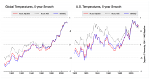
Having worked with many of the scientists in question, I can say with certainty that there is no grand conspiracy to artificially warm the earth; rather, scientists are doing their best to interpret large datasets with numerous biases such as station moves, instrument changes, time of observation changes, urban heat island biases, and other so-called inhomogenities that have occurred over the last 150 years. Their methods may not be perfect, and are certainly not immune from critical analysis, but that critical analysis should start out from a position of assuming good faith and with an understanding of what exactly has been done.
This will be the first post in a three-part series examining adjustments in temperature data, with a specific focus on the U.S. land temperatures. This post will provide an overview of the adjustments done and their relative effect on temperatures. The second post will examine Time of Observation adjustments in more detail, using hourly data from the pristine U.S. Climate Reference Network (USCRN) to empirically demonstrate the potential bias introduced by different observation times. The final post will examine automated pairwise homogenization approaches in more detail, looking at how breakpoints are detected and how algorithms can tested to ensure that they are equally effective at removing both cooling and warming biases.
Why Adjust Temperatures?
There are a number of folks who question the need for adjustments at all. Why not just use raw temperatures, they ask, since those are pure and unadulterated? The problem is that (with the exception of the newly created Climate Reference Network), there is really no such thing as a pure and unadulterated temperature record. Temperature stations in the U.S. are mainly operated by volunteer observers (the Cooperative Observer Network, or co-op stations for short). Many of these stations were set up in the late 1800s and early 1900s as part of a national network of weather stations, focused on measuring day-to-day changes in the weather rather than decadal-scale changes in the climate.
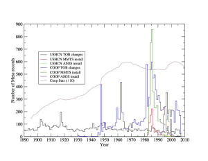
Nearly every single station in the network in the network has been moved at least once over the last century, with many having 3 or more distinct moves. Most of the stations have changed from using liquid in glass thermometers (LiG) in Stevenson screens to electronic Minimum Maximum Temperature Systems (MMTS) or Automated Surface Observing Systems (ASOS). Observation times have shifted from afternoon to morning at most stations since 1960, as part of an effort by the National Weather Service to improve precipitation measurements.
All of these changes introduce (non-random) systemic biases into the network. For example, MMTS sensors tend to read maximum daily temperatures about 0.5 C colder than LiG thermometers at the same location. There is a very obvious cooling bias in the record associated with the conversion of most co-op stations from LiG to MMTS in the 1980s, and even folks deeply skeptical of the temperature network like Anthony Watts and his coauthors add an explicit correction for this in their paper.
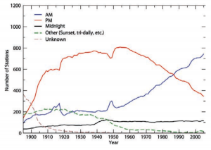
Time of observation changes from afternoon to morning also can add a cooling bias of up to 0.5 C, affecting maximum and minimum temperatures similarly. The reasons why this occurs, how it is tested, and how we know that documented time of observations are correct (or not) will be discussed in detail in the subsequent post. There are also significant positive minimum temperature biases from urban heat islands that add a trend bias up to 0.2 C nationwide to raw readings.
Because the biases are large and systemic, ignoring them is not a viable option. If some corrections to the data are necessary, there is a need for systems to make these corrections in a way that does not introduce more bias than they remove.
What are the Adjustments?
Two independent groups, the National Climate Data Center (NCDC) and Berkeley Earth (hereafter Berkeley) start with raw data and use differing methods to create a best estimate of global (and U.S.) temperatures. Other groups like NASA Goddard Institute for Space Studies (GISS) and the Climate Research Unit at the University of East Anglia (CRU) take data from NCDC and other sources and perform additional adjustments, like GISS’s nightlight-based urban heat island corrections.
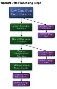
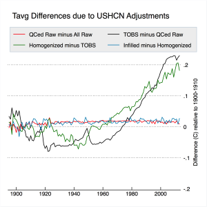
This post will focus primarily on NCDC’s adjustments, as they are the official government agency tasked with determining U.S. (and global) temperatures. The figure below shows the four major adjustments (including quality control) performed on USHCN data, and their respective effect on the resulting mean temperatures.
NCDC starts by collecting the raw data from the co-op network stations. These records are submitted electronically for most stations, though some continue to send paper forms that must be manually keyed into the system. A subset of the 7,000 or so co-op stations are part of the U.S. Historical Climatological Network (USHCN), and are used to create the official estimate of U.S. temperatures.
Quality Control
Once the data has been collected, it is subjected to an automated quality control (QC) procedure that looks for anomalies like repeated entries of the same temperature value, minimum temperature values that exceed the reported maximum temperature of that day (or vice-versa), values that far exceed (by five sigma or more) expected values for the station, and similar checks. A full list of QC checks is available here.
Daily minimum or maximum temperatures that fail quality control are flagged, and a raw daily file is maintained that includes original values with their associated QC flags. Monthly minimum, maximum, and mean temperatures are calculated using daily temperature data that passes QC checks. A monthly mean is calculated only when nine or fewer daily values are missing or flagged. A raw USHCN monthly data file is available that includes both monthly values and associated QC flags.
The impact of QC adjustments is relatively minor. Apart from a slight cooling of temperatures prior to 1910, the trend is unchanged by QC adjustments for the remainder of the record (e.g. the red line in Figure 5).
Time of Observation (TOBs) Adjustments
Temperature data is adjusted based on its reported time of observation. Each observer is supposed to report the time at which observations were taken. While some variance of this is expected, as observers won’t reset the instrument at the same time every day, these departures should be mostly random and won’t necessarily introduce systemic bias. The major sources of bias are introduced by system-wide decisions to change observing times, as shown in Figure 3. The gradual network-wide switch from afternoon to morning observation times after 1950 has introduced a CONUS-wide cooling bias of about 0.2 to 0.25 C. The TOBs adjustments are outlined and tested in Karl et al 1986 and Vose et al 2003, and will be explored in more detail in the subsequent post. The impact of TOBs adjustments is shown in Figure 6, below.
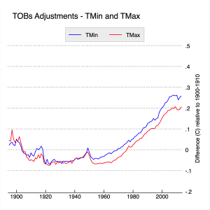
TOBs adjustments affect minimum and maximum temperatures similarly, and are responsible for slightly more than half the magnitude of total adjustments to USHCN data.
Pairwise Homogenization Algorithm (PHA) Adjustments
The Pairwise Homogenization Algorithm was designed as an automated method of detecting and correcting localized temperature biases due to station moves, instrument changes, microsite changes, and meso-scale changes like urban heat islands.
The algorithm (whose code can be downloaded here) is conceptually simple: it assumes that climate change forced by external factors tends to happen regionally rather than locally. If one station is warming rapidly over a period of a decade a few kilometers from a number of stations that are cooling over the same period, the warming station is likely responding to localized effects (instrument changes, station moves, microsite changes, etc.) rather than a real climate signal.
To detect localized biases, the PHA iteratively goes through all the stations in the network and compares each of them to their surrounding neighbors. It calculates difference series between each station and their neighbors (separately for min and max) and looks for breakpoints that show up in the record of one station but none of the surrounding stations. These breakpoints can take the form of both abrupt step-changes and gradual trend-inhomogenities that move a station’s record further away from its neighbors. The figures below show histograms of all the detected breakpoints (and their magnitudes) for both minimum and maximum temperatures.
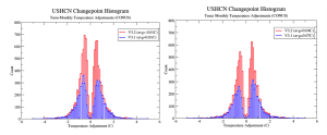
While fairly symmetric in aggregate, there are distinct temporal patterns in the PHA adjustments. The single largest of these are positive adjustments in maximum temperatures to account for transitions from LiG instruments to MMTS and ASOS instruments in the 1980s, 1990s, and 2000s. Other notable PHA-detected adjustments are minimum (and more modest maximum) temperature shifts associated with a widespread move of stations from inner city rooftops to newly-constructed airports or wastewater treatment plants after 1940, as well as gradual corrections of urbanizing sites like Reno, Nevada. The net effect of PHA adjustments is shown in Figure 8, below.
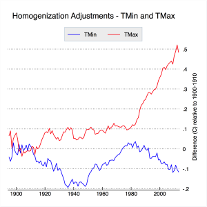
The PHA has a large impact on max temperatures post-1980, corresponding to the period of transition to MMTS and ASOS instruments. Max adjustments are fairly modest pre-1980s, and are presumably responding mostly to the effects of station moves. Minimum temperature adjustments are more mixed, with no real century-scale trend impact. These minimum temperature adjustments do seem to remove much of the urban-correlated warming bias in minimum temperatures, even if only rural stations are used in the homogenization process to avoid any incidental aliasing in of urban warming, as discussed in Hausfather et al. 2013.
The PHA can also effectively detect and deal with breakpoints associated with Time of Observation changes. When NCDC’s PHA is run without doing the explicit TOBs adjustment described previously, the results are largely the same (see the discussion of this in Williams et al 2012). Berkeley uses a somewhat analogous relative difference approach to homogenization that also picks up and removes TOBs biases without the need for an explicit adjustment.
With any automated homogenization approach, it is critically important that the algorithm be tested with synthetic data with various types of biases introduced (step changes, trend inhomogenities, sawtooth patterns, etc.), to ensure that the algorithm will identically deal with biases in both directions and not create any new systemic biases when correcting inhomogenities in the record. This was done initially in Williams et al 2012 and Venema et al 2012. There are ongoing efforts to create a standardized set of tests that various groups around the world can submit homogenization algorithms to be evaluated by, as discussed in our recently submitted paper. This process, and other detailed discussion of automated homogenization, will be discussed in more detail in part three of this series of posts.
Infilling
Finally we come to infilling, which has garnered quite a bit of attention of late due to some rather outlandish claims of its impact. Infilling occurs in the USHCN network in two different cases: when the raw data is not available for a station, and when the PHA flags the raw data as too uncertain to homogenize (e.g. in between two station moves when there is not a long enough record to determine with certainty the impact that the initial move had). Infilled data is marked with an “E” flag in the adjusted data file (FLs.52i) provided by NCDC, and its relatively straightforward to test the effects it has by calculating U.S. temperatures with and without the infilled data. The results are shown in Figure 9, below:
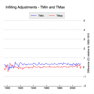
Apart from a slight adjustment prior to 1915, infilling has no effect on CONUS-wide trends. These results are identical to those found in Menne et al 2009. This is expected, because the way NCDC does infilling is to add the long-term climatology of the station that is missing (or not used) to the average spatially weighted anomaly of nearby stations. This is effectively identical to any other form of spatial weighting.
To elaborate, temperature stations measure temperatures at specific locations. If we are trying to estimate the average temperature over a wide area like the U.S. or the Globe, it is advisable to use gridding or some more complicated form of spatial interpolation to assure that our results are representative of the underlying temperature field. For example, about a third of the available global temperature stations are in U.S. If we calculated global temperatures without spatial weighting, we’d be treating the U.S. as 33% of the world’s land area rather than ~5%, and end up with a rather biased estimate of global temperatures. The easiest way to do spatial weighting is using gridding, e.g. to assign all stations to grid cells that have the same size (as NASA GISS used to do) or same lat/lon size (e.g. 5×5 lat/lon, as HadCRUT does). Other methods include kriging (used by Berkeley Earth) or a distance-weighted average of nearby station anomalies (used by GISS and NCDC these days).
As shown above, infilling has no real impact on temperature trends vs. not infilling. The only way you get in trouble is if the composition of the network is changing over time and if you do not remove the underlying climatology/seasonal cycle through the use of anomalies or similar methods. In that case, infilling will give you a correct answer, but not infilling will result in a biased estimate since the underlying climatology of the stations is changing. This has been discussed at length elsewhere, so I won’t dwell on it here.
I’m actually not a big fan of NCDC’s choice to do infilling, not because it makes a difference in the results, but rather because it confuses things more than it helps (witness all the sturm und drang of late over “zombie stations”). Their choice to infill was primarily driven by a desire to let people calculate a consistent record of absolute temperatures by ensuring that the station composition remained constant over time. A better (and more accurate) approach would be to create a separate absolute temperature product by adding a long-term average climatology field to an anomaly field, similar to the approach that Berkeley Earth takes.
Changing the Past?
Diligent observers of NCDC’s temperature record have noted that many of the values change by small amounts on a daily basis. This includes not only recent temperatures but those in the distant past as well, and has created some confusion about why, exactly, the recorded temperatures in 1917 should change day-to-day. The explanation is relatively straightforward. NCDC assumes that the current set of instruments recording temperature is accurate, so any time of observation changes or PHA-adjustments are done relative to current temperatures. Because breakpoints are detected through pair-wise comparisons, new data coming in may slightly change the magnitude of recent adjustments by providing a more comprehensive difference series.
When breakpoints are removed, the entire record prior to the breakpoint is adjusted up or down depending on the size and direction of the breakpoint. This means that slight modifications of recent breakpoints will impact all past temperatures at the station in question though a constant offset. The alternative to this would be to assume that the original data is accurate, and adjusted any new data relative to the old data (e.g. adjust everything in front of breakpoints rather than behind them). From the perspective of calculating trends over time, these two approaches are identical, and its not clear that there is necessarily a preferred option.
Hopefully this (and the following two articles) should help folks gain a better understanding of the issues in the surface temperature network and the steps scientists have taken to try to address them. These approaches are likely far from perfect, and it is certainly possible that the underlying algorithms could be improved to provide more accurate results. Hopefully the ongoing International Surface Temperature Initiative, which seeks to have different groups around the world send their adjustment approaches in for evaluation using common metrics, will help improve the general practice in the field going forward.

